Introduction to cold junction theory
When
accurate thermocouple measurements are required, it is common
practice to reference both legs to copper lead wire at the ice
point so that copper leads may be connected to the emf readout
instrument due to the cold junction. This procedure avoids the generation of thermal emfs
at the terminals of the readout instrument. Changes in reference
junction temperature influence the output signal and practical
instruments must be provided with a means to cancel this potential
source of error.
The EMF generated is dependent on a difference
in temperature in the junction, so in order to make a measurement the reference
must be known. This is shown schematically in Fig. #1 and can
be accomplished by placing the reference junction in an ice water
bath at a constant 0°C (32°F). Because ice baths are often inconvenient
to maintain and not always practical, several alternate methods
are often employed.
Techniques to compensates the cold junction
Electrical Bridge Method
This method usually employs a self-compensating cold junction
electrical bridge circuit as shown in Figure 2. This system incorporates
a temperature sensitive resistance element (RT), which is in one
leg of the bridge network and thermally integrated with the cold
junction (T2). The bridge is usually energized from a mercury
battery or stable d.c. power source. The output voltage is proportional
to the unbalance created between the pre-set equivalent reference
temperature at (T2) and the hot junction (T1). In this system,
the reference temperature of 0° or 32°F may be chosen.
As
the ambient temperature surrounding the cold junction (T2) varies,
a thermally generated voltage appears and produces an error in
the output. However, an automatic equal and opposite voltage is
introduced in series with the thermal error. This cancels the
error and maintains the equivalent reference junction temperature
over a wide ambient temperature range with a high degree of accuracy.
By integrating copper leads with the cold junction, the thermocouple
material itself is not connected to the output terminal of the
measurement device, thereby eliminating secondary errors.
Thermoelectric refriferation method
The Omega¨ TRC Thermoelectric
ice pointTM Reference Chamber relies on the actual equilibrium
of ice and distilled, deionized water and atmospheric pressure
to maintain several reference wells at precisely 0°C. The wells
are extended into a sealed cylindrical chamber containing pure
distilled, deionized water.
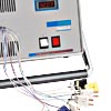 Portable Ice Point™ Calibration Reference Chamber
The new ice point™ reference chamber TRCIII-A is the latest addition to OMEGA’s fine line of calibration reference instrumentation. The TRCIII-A ice point™ reference chamber relies on the equilibrium of ice and distilled, deionized water at atmospheric pressure to maintain six reference wells at precisely 0°C.
The chamber outer walls are cooled
by thermoelectric cooling elements to cause freezing of the water
in the cell to work as a cold junction reference. The increase in volume produced by freezing an ice
shell on the cell wall is sensed by the expansion of a bellows
which operates a microswitch, de-energizing the cooling element.
The alternate freezing and thawing of the ice shell accurately
maintains a 0°C environment around the reference wells. An application
schematic is shown in Fig. #3.
Completely
automatic operation eliminates the need for frequent attention
required of common ice baths. Thermocouple readings may be made
directly from ice point reference tables without making corrections for reference
junction temperature.
Any combination of thermocouples may be
used with this instrument by simply inserting the reference junctions
in the reference wells. Calibration of other type temperature
sensors at 0°C may be performed as well. Heated oven references:
The double-oven type employs two temperature-controlled ovens
to simulate ice-point reference temperatures as shown in Fig.
4. Two ovens are used at different temperatures to give the equivalent
of a low reference temperature differing from the temperature
of either oven.
For example, leads from a type K thermocouple
probe are connected with a 150° oven to produce a Chromega¨-Alomega¨
and an Alomega-Chromega junction at 150°F (2.66 mV each).
The
voltage between the output wires of the first oven will be twice
2.66 mV or 5.32 mV. To compensate for this voltage level, the
output leads (Chromega and Alomega) are connected to copper leads
within a second oven maintained at 265.5°F. This is the precise
temperature at which Chromega-Copper and Alomega-Copper produce
a bucking voltage of differential of 5.32 mV.
Thus, this voltage
cancels out the 5.32 mV differential from the first oven leaving
0 mV at the Copper output terminals. This is the voltage equivalent
of 32°F (0°C).
 CLOSE
CLOSE